Southern Wet Ash Swamp - WFs57
Forest description
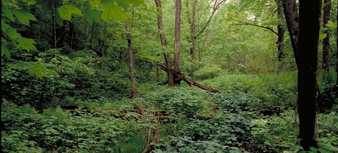
Wet hardwood forests on mucky or peaty soils in areas of groundwater seepage. Usually present on level river terraces at bases of steep slopes.
Community description
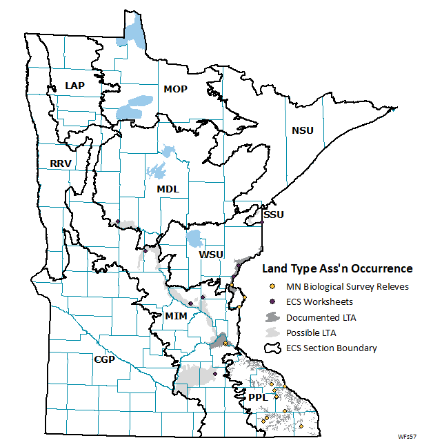
WFs57 forested swamps are a relatively uncommon hardwood community located in southeast and east-central Minnesota (see map; 17 relevés, 9 ECS worksheets). Nearly all observations of the WFs57 community are found in the Paleozoic Plateau (PPL) section. Other observations are along major river corridors of the Mississippi and St. Croix Rivers.
Distribution in Minnesota
Vegetation structure and composition
Description is based on summary of vegetation data from 24 plots (relevés)
- Ground-layer is characterized by raised peaty hummocks, with open pools and rivulets in seepage areas. Wetland species such as common marsh marigold (Caltha palustris) and fowl manna grass (Glyceria striata) are common in wet areas, with touch-me-nots (Impatiens spp.), Virginia creepers (Parthenocissus spp.), jack-in-the-pulpit (Arisaema triphyllum), wood nettle (Laportea canadensis), wild geranium (Geranium maculatum), tall coneflower (Rudbeckia laciniata), and other mesic or wet-mesic forest species present on hummocks. Skunk cabbage (Symplocarpus foetidus) is often present in seepage zones.
- Shrub-layer is sparse (5-25% cover). Black ash seedlings or saplings are almost always present, often with chokecherry (Prunus virginiana), wild black currant (Ribes americanum), and nannyberry (Viburnum lentago).
- Subcanopy, when present, is patchy to interrupted (25-75% cover) and generally not well differentiated from canopy.
- Canopy is patchy to interrupted and dominated by black ash, often with other hardwood species, especially basswood, sugar maple, and American elm. Yellow birch is sometimes abundant.
Landscape setting and soils
WFs57 occurs on strongly rolling to steeply dissected terrain where there is sufficient relief for groundwater to upwell in springs or in broad discharge zones. Most often these seepage areas are present at the contact between steep bedrock slopes and alluvial river valley bottoms; less often, they develop in regions of deep glacial drift where groundwater flows through highly permeable aquifers and emerges at the ground surface. In all settings, springheads and rivulets with continuously flowing cold groundwater are evident. Parent material is silty colluvium or alluvium capped by mucky peat. The organic cap is often thin and discontinuous in the southeastern blufflands, and thicker to the north, where peat depths can exceed 40in (100cm). The underlying mineral soil is gray, indicating permanent saturation. Soils are poorly to very poorly drained. Soil-moisture regime is very moist to moderately wet. (WSU, MIM)
Tree suitability
The suitability index is our estimate of a tree's ability to compete with all plants in a particular NPC Class without silvicultural assistance. The data come from forests approaching rotation age or older. The raw index is based upon the product of percent presence and mean cover-when-present (below) within the set of relevés classified as that NPC. Plants are ranked by their raw index and the full rank order is partitioned into 5 equal groups of plants and re-scaled to yield the suitability index ranging from 1 to 5. This is done so that the indices can be compared within the NPC (below) or with other NPC classes (statewide suitability table[AJ(1]).
It is important to note that the table presented below is a landscape summary of how trees perform on average in a NPC Class. At the stand-scale current stocking and any knowledge of the stand's disturbance/management history should inform how the suitability table can be used. Discussion of stand-scale application of the table follows below the table.
The table is also useful at the landscape-scale when there are restoration or conservation needs for the NPC Class itself, or when forest plan directives call for a management emphasis of a particular species. Species with a high suitability index that are not currently present on the site can be introduced to the site with less risk than species with a lower index.
- Learn more about tree suitability
A tree species is 'suited' to a site when its physical and genetic makeup allow for it to survive and reproduce given the constraints of a site's physical environment AND co-occurring vegetation. Ecologists call this the 'realized niche' of a tree. Our suitability index is based upon the assumption that a tree is highly suited to a site when we see it often and in great abundance in its Native Plant Community Class.
These tables are intended to help foresters decide which tree species to silviculturally favor or introduce on sites that have been classified using the Field Guides to the Native Plant Communities of Minnesota1. Trees with excellent suitability should grow well with very little silvicultural treatment other than providing the correct light and seedbed environments for establishment and recruitment. Trees with poorer suitability for a site can be grown to meet specific objectives, but the forester should expect progressive increases in cost and risk for trees with good to fair to poor suitability rankings. The underlying assumption for using these tables is that when trees are naturally suited to their site, they are vigorous. Vigor should translate to superior quality, resistance to disease, capacity for natural regeneration, and the ability to withstand fluctuations in climate.
Suitability Index
Suitability is a mathematical calculation. The data for this calculation come from 6,303 vegetation plots that have been classified as belonging to one of 54 forested NPCs. Two metrics -- commonness and local abundance -- are the elements of suitability.A plant is 'suited' to a NPC when we often find it there. Percent presence was our metric of commonness. Similarly, a plant is 'suited' to a NPC when it tends to occur in abundance when present. Mean percent cover-when-present was our metric of local abundance. The suitability index is the product of percent presence and mean percent cover-when-present.
Example: Of the 6,306 sample plots, 757 were classified as Northern Mesic Hardwood Forest (MHn35). Basswood trees occur in 483 of the 757 plots. Thus, its percent presence as a tree is (483/757)*100= 63.8%. The mean cover of basswood trees on those 757 plots is 16.5%. Thus, its raw suitability index is 63.8*16.5=1,053. There are 158 species with >3% presence in MHn35 forests and basswood's rank order on a scale of 1-5 is 4.8, its standardized suitability index. The index is standardized so that basswood's suitability can be compared among different NPC classes.
| Tree Type | Presence as Tree | Mean Cover When Present | Suitability Index | Crop Tree Potential |
|---|
- Legend for tree suitability values
Suitability index values Crop Tree Potential Color 4.0 - 5.0 Excellent Green 3.0 – 3.99 Good Blue 2.0 – 2.99 Fair Yellow
In general, trees with higher suitability indices are better adapted to the hydrologic regime of WFs57 sites than trees with lower indices. Several species are adapted to these sites, with 11 species having a fair, good, or excellent suitability. Black ash, basswood, sugar maple, paper birch, American elm, yellow birch, and peach-leaved willow are ranked as having excellent suitability by virtue of their frequent occurrence and moderately high cover-when-present on WFs57 sites. In spite of some tree diversity, only black ash commonly forms the cover type. In the absence of large American elms, black ash dominates all growth-stages. All other suited species become more prevalent as stands age about the persistent core of black ash. White pine and bur oak are ranked as having good suitability, and they can occur in abundance on the more terrestrial inclusions in and around WFs57 wetlands. Red elm and silver maple are ranked as having just fair suitability and they occur mostly because WFs57 sites are often adjacent to floodplain and terrace forests where red elm and silver maple are common trees. WFs57 wetlands are of little commercial interest because they are inoperable due to groundwater discharge that prevents and deep frost from forming. These forests have great conservation value, and harbor some of the State’s rarer plants. Any silvicultural intervention should be done only for restorative purposes.
Tree response to climate change
Land managers are adapting management strategies to position the forested landscape into one that will be resilient in Minnesota's changing climate. Trends in climate data have shown that Minnesota is getting warmer and wetter, please view the DNR's climate trends webpage for more information. Differences among the 52 forested NPCs are related very much to water availability for trees and understory plants. Forested communities have different capacities for interception, infiltration, storage, and runoff, thus we expect them to react differently to changes in the hydrologic regime -- whatever that may be.
Climate change considerations for forest management can be thought of as a 'funnel' that guides a landowner to make decisions at a successively narrower spatial extent from landscape, to region, then site. The land manager must evaluate information for an entire ecosystem (e.g., hydrology, soils, and forest health) and how manipulations to that ecosystem may be reflected in the tree species present. Generally, the goal is to select tree species that will be resilient to the changing climate and survive through a full stand rotation.
The widest part of the funnel is the landscape-level, here we keep in mind the full suite of species that currently exist in the forested landscape, those that may arrive, and those who's importance across the landscape may decrease. To understand climate change at this broad level read the Minnesota Forest Ecosystem Vulnerability Assessment and Synthesis, where you will learn about how a warmer and wetter climate will impact ecosystem functions and operability concerns (e.g., frozen ground conditions, length of growing season, and prevalence of drought).
The middle part of the funnel is the region-level. At this stage of climate change analysis researchers have defined changes land managers can assess for System Groups (i.e. forest types), instead of impacts to forests as a whole. The Climate Change Field Guide for Northern Minnesota Forests highlights how changes in precipitation and temperature may result in ecosystem changes such as hydrology modifications, increase/decrease in frost days, and drought stress, and apply those concepts to the species adapted to our System Groups. Regionally, land managers can also start brainstorming how the System characteristics may make it well suited for adaptation or vulnerable to climate stressors. Please view the Site-level Considerations for the six main forested systems in the Climate Change Field Guide for Northern Minnesota Forests publication to gain knowledge about site characteristics that would increase or decrease climate risk.
The smallest spatial extent a land manager must think about for climate change is the site-level. Here users must apply the regional Site-level Considerations with the conditions currently found on site. The land manager should assess the climate change risk and how a prescription may be modified in order to favor or disfavor certain tree species. The information provided below is our analysis of the competitive advantage a single species has within a community if the integrity of the community is expected to be maintained into the future. Overall, some of the species we present having a higher heat/moisture tolerance within the community may well be expected to diminish in habitat suitability across the region due to climate change. The species listed also do not represent any tree species changes as forests adapt through time.
It is important to remember that individual site conditions will vary and opportunities to create resilient forests will be a site-by-site analysis. Overall, keeping the full complement of suitable trees on-site is a good hedge against future climate uncertainty.
- Learn more about tree response to climate change
Incorporating climate change information into a site prescription can be a complicated web of understanding information at multiple scales. Most climate change prediction data answers questions about how a tree species will perform across a broad heterogeneous landscape, but decisions about species risk need to be made for individual sites. The following guides in the Learn More expansion provide useful information about vulnerabilities across forested-Minnesota. Please pay close attention to the Climate Change Field Guide as it highlights System Group-specific information and site-level considerations for each NPC System within the Laurentian Mixed Forest Province. Lastly, tree species concerns are neatly explained in the Northwoods Tree Handouts. All of these resources together can help a forester develop the desired future conditions for a forest.
Synecological score calculations
An analysis of habitat range climate data was used to assign and adjust synecological scores for our plants with regard to moisture (M) and temperature (H). The scores range from 1 (dry/cool) to 5 (wet/warm). The difference between a plant's individual synecological score and the mean synecological score of its community provides some insight as to whether that plant would benefit or suffer should its local environment become warmer or wetter.Example: For each of the 256 MHn35 vegetation plots, the M score of all component plants was summed and averaged to yield a score for each plot. Then the plot scores were summed and averaged to yield an M score for the community, which in this case was 2.3. The adjusted M score for basswood is 2.01, which is drier than 2.3. Thus, we assume that basswood would benefit from a slightly drier conditions. Similarly, the H score for basswood is 4.03, which is substantially warmer than the 2.9 mean for the MHn35 community, which suggests basswood would greatly benefit if MHn35 sites get warmer.
For more information about synecological scores, please view the following references:
Bakuzis, E.V. and Kurmis, V. 1978. Provisional list of synecological coordinates and selected ecographs of forest and other plant species in Minnesota. Staff Series Paper 5. Department of Forest Resources, University of Minnesota. St. Paul, MN.
Brand, G.J., and Almendinger, J.C. 1992. Synecological coordinates as indicators of variation in red pine productivity among TWINSPAN classes: A case Study. Research Paper NC-310. North Central Forest Experiment Station, U.S. Department of Agriculture, St. Paul, MN.For information about regional forest vulnerability, please view Minnesota Forest Ecosystem Vulnerability Assessment and Synthesis:
Handler, Stephen; Duveneck, Matthew J.; Iverson, Louis; Peters, Emily; Scheller, Robert M.; Wythers, Kirk R.; Brandt, Leslie; Butler, Patricia; Janowiak, Maria; Shannon, P. Danielle; Swanston, Chris; Barrett, Kelly; Kolka, Randy; McQuiston, Casey; Palik, Brian; Reich, Peter B.; Turner, Clarence; White, Mark; Adams, Cheryl; D'Amato, Anthony; Hagell, Suzanne; Johnson, Patricia; Johnson, Rosemary; Larson, Mike; Matthews, Stephen; Montgomery, Rebecca; Olson, Steve; Peters, Matthew; Prasad, Anantha; Rajala, Jack; Daley, Jad; Davenport, Mae; Emery, Marla R.; Fehringer, David; Hoving, Christopher L.; Johnson, Gary; Johnson, Lucinda; Neitzel, David; Rissman, Adena; Rittenhouse, Chadwick; Ziel, Robert. 2014. Minnesota forest ecosystem vulnerability assessment and synthesis: a report from the Northwoods Climate Change Response Framework project. Gen. Tech. Rep. NRS-133. Newtown Square, PA; U.S. Department of Agriculture, Forest Service, Northern Research Station. 228 p.
Available online at https://www.fs.usda.gov/nrs/pubs/gtr/gtr_nrs133.pdfFor information about site-level considerations and vulnerabilities for NPC System Groups, please view the Climate Change Field Guide for Northern Minnesota Forests:
Handler, S., K. Marcinkowski, M. Janowiak, and C. Swanston. 2017. Climate change field guide for northern Minnesota forests: Site-level considerations and adaptation. USDA Northern Forests Climate Hub Technical Report #2. University of Minnesota College of Food, Agricultural, and Natural Resource Sciences, St. Paul, MN. 88p. Available at www.forestadaptation.org/MN_field_guideIndividual tree species adaptation characteristics and climate change projections across subsection-level areas can be found here:
https://forestadaptation.org/learn/resource-finder/climate-change-projections-tree-species-northwoods-mn-wi-mi
Climate in Minnesota has been getting warmer and wetter. If this trend continues the descriptions in the table forecast the direction and magnitude how we expect WFs57 trees to respond. The responses of “slight” or “significant” increases/decreases represents a full unit departure from the mean synecological score for the WFs57 community.
| Tree Type | Response to warmer climate | Response to wetter climate |
|---|
Tree establishment and recruitment
The vertical structure of releves was used to interpret the ability of trees to establish themselves and recruit to taller strata under the canopy of a mature forest and on seedbeds associated with older forests. The goal was to develop an appreciation of which trees are capable of developing enough advance regeneration to fully stock a future stand by natural regeneration. For trees with modest advance regeneration, we wanted to figure out if the problem seems to be related to poor establishment or poor recruitment -- issues that can be silviculturally resolved. For trees with little or no advance regeneration but good or excellent suitability as a tree, we assume that even-aged systems would be required to perpetuate them in that community.
Establishment and recruitment indices are calculations designed to estimate how a tree performs in different size classes with no silvicultural assistance:
1. small regenerant <10cm tall, R-index
2. seedling 10cm -- 2m, SE-index
3. sapling 2m -- 10m, SA-index
4. tree >10m, T-index
The index is the product of percent presence, mean percent cover-when-present, and mean number of reported strata. The index is re-scaled to run from 0 to 5 so that suitability can be compared among different NPCs.
- Learn more about tree establishment and recruitment indices
The tree height data from releves was transformed into 4 standard height strata: regenerants <10cm tall, seedlings 10cm -- 2 m tall, saplings 2 -- 10m tall, and trees >10m. These height breaks were used because they are the most frequently used on releves to describe the natural structural breaks in forests. Still, some releves report strata that span our standard height seams and we had to apportion the presence of the tree and its percent cover into our standard classes. This was done by splitting the reported strata into the 8 individual height classes and evenly splitting the cover among the classes. For example, sugar maple reported in a D3-6 layer (0.5-20m) comprises four individual height classes that need to contribute cover to our standard seedling, sapling, and tree strata. The cover of sugar maple in that stratum was class 3 (25-50% cover). Using the mid-point rule as for suitability (see above), cover class 3 is converted to 37.5%, and the apportionment is 37.5% / 4 = 9.37% cover awarded for sugar maple in each height class. After cover was awarded to all individual height classes in a releve, they were then lumped into the standard strata and the individual covers summed.
For each standard stratum we calculated an index of 'regeneration success' for the tree species. We settled on three measures of success:
First, trees were considered successful if they were common in a particular stratum. Presence is our measure of stratum commonness, and below is how seedling presence was calculated. The parallel calculation was done also for regenerants, saplings, and trees.
SE Presence = (# of releves with the tree present as a seedling / total # of releves for the community) * 100
Second, trees were considered successful if we found them to be abundant in a particular stratum. Mean cover-when-present (MCWP) was our measure of stratum abundance, and below is how seedling MCWP was calculated. The parallel calculation was done also for regenerants, saplings, and trees.
SE MCWP = sum of all seedling cover of tree / number of releves with the tree present as a seedling
Third, trees were considered successful recruiters if we often found it in multiple strata. As a measure of recruitment complexity we calculated the mean number of strata when present (MSWP) reported in the original releves (not our standard strata) for a species. We used this number as a weighting factor to help segregate species that develop a presence in many layers from those that don't develop a lot of strata because they probably need some kind of disturbance to develop an understory cohort.
MSWP = sum of all reported strata for a species / number of releves in which the species occurs
From these three measures of stratum success we calculated the raw recruitment index by multiplying the numbers together. Below is how the raw seedling index was calculated.
Raw SE Index = SE presence * SE MCWP * SE MSWP
For each stratum -- regenerants, seedlings, saplings, and trees -- the ranges of raw index scores are different and not comparable between strata and between communities. To allow comparison, the raw scores were ranked and then re-scaled so that the lowest raw score was zero and the maximum was five.
The indices of regeneration were placed into classes as for suitability so that in tables, foresters can quickly identify the species that tend to have poor, fair, good, or excellent regeneration in mature forests that have not been silviculturally manipulated in the recent past.
Regeneration Index Equivalent Percentile Descriptor 0-1 0-20% none 1-2 20-40% Poor Suitability 2-3 40-60% Fair Suitability 3-4 60-80% Good Suitability 4-5 80-100% Excellent Suitability
| Tree Type | Presence R/SE/SA | R-index | SE-index | SA-index | T-index |
|---|
- Legend for tree establishment values
Index values Rating Color 4.0 - 5.0 Excellent Green 3.0 – 3.99 Good Blue 2.0 – 2.99 Fair Yellow 1.0 – 1.99 Fair Orange 0.0 – 0.99 Fair White
In general, trees with high understory presence and excellent R-, SE-, and SA-indices can be depended upon to produce enough advance regeneration to stock a stand after removal of canopy trees. In WFs57 forests black ash and American elm are almost always present in usable abundance; however American elm is not long-lived after attaining the height of 10m. At maturity black ash dominates both the understory and overstory, and the forest is self-sustaining.
Trees with excellent R-index values have no problem establishing on an undisturbed forest floor in mature WFs57 forests. Only black ash and American elm readily establish by seed without any seedbed preparation. This indicates a germination need that is not fully met in a mature WFs57 forest. The need is often species-specific, thus silvicultural improvement requires knowledge of the tree’s silvics and its competitive context following silvicultural treatment in WFs57 forests. Common germination hurdles in WFs57 forests are: prolonged inundation in the spring, insufficient light/heat due to proximal shade from shrubs and subcanopy trees, poor ability to use ammonium as a nitrogen source, lack of nurse logs, and lack of seed source.
Trees with excellent SE- and SA-index need no silvicultural assistance recruiting to tree size in an unmanaged forest. Only black ash and American elm do this in WFs57 forests. American elm has some difficulty recruiting to heights much over 10m, most likely because at that height it is first susceptible to Dutch elm disease. Trees with either a good or fair SE- or SA-index would likely benefit from intermediate silvicultural treatment as long as establishment isn’t a problem. If the SE-index is the lower of the two then early survival and growth is the issue, and treatments like cleaning and spacing may help to diminish proximal competition. This is clearly the case for sugar maple, basswood, and yellow birch. Red elm may fit this pattern, but its R-index is also low, suggesting that establishment and early growth are both a problem. If the SA-index is the lower of the two then the issue is most likely sufficient light as the trees try to emerge from the shrub layer, and overhead release may help to promote the advance regeneration. This may be the case for bur oak. Trees like paper birch, silver maple, white pine, and peach-leaved willow with very poor understory indices generally need to be regenerated under more open conditions where recruitment under a canopy isn’t an issue. Their occasional occurrence in WFs57 forests is spurious in that these trees occur in adjacent upland and floodplain forests and upon rare occasion will occupy a large gap.
These forests have great conservation value, and harbor some of the State’s rarer plants. Any silvicultural intervention should be done only for restorative purposes.
Natural disturbance
Understanding natural disturbance regimes is prerequisite for designing silvicultural systems and treatments that emulate natural processes. Theoretically, 'natural' treatments favor trees adapted to the site, conserve local gene pools by relying on natural regeneration, maintain native plants in the understory, are less risky than agricultural approaches, and cheaper to implement. Because clear-cutting and other stand-regenerating systems are so often employed, it is important to determine which NPCs were maintained by stand-replacing disturbances and, further, to estimate the natural rotation. For many NPCs the natural rotation far exceeds commercial rotation, and this requires us to look to other silvicultural strategies for harvest and regeneration. Thus, we must also estimate the frequency and intensity of disturbances that maintain these kinds of forest communities.
Natural rotation of catastrophic and maintenance disturbances were calculated from Public Land Survey (PLS) records. The records provide a point-in-time estimate (ca. 1846-1908 AD) of just how much of the historic landscape was recently disturbed by fire, windthrow, or gap-forming events such as surface fires, disease pockets, etc. To some extent these regional trends can be applied to management at the stand-scale. The kind of natural disturbance can inform site preparation; the comparative frequency of stand-replacement and maintenance events informs canopy retention and entry schedules/rotation.
Learn more about calculating natural disturbance rotations
Natural Disturbance Regimes
The goal of the PLS analysis was to estimate the rotation of stand-replacement and maintenance disturbances unique to each NPC class. The surveyors explicitly described burned and windthrown land when working within the forested regions of Minnesota. When in the prairie region and especially along the prairie/forest border, the surveyors used a variety of terms to describe wooded vegetation understood to be maintained by frequent disturbance. Most often this was fire, but in some regions wind was important as well. Thus, geographic context is an important consideration when trying to determine if a surveyor's comments are indicating that the corner was 1) undisturbed, 2) catastrophically disturbed, or 3) recently affected by a less intense, maintenance disturbance. Placing corners in these three categories is the critical step that allows the calculation of disturbance regimes. To get at this, we must understand the surveyor's physiognomic descriptions of the vegetation at the corners: prairie, grove, bottoms, barrens, burned lands, windthrown timber, etc. Our rules for assessing disturbance at survey corners were individually set for each physiognomic vegetation type across the state.
Stocking (i.e., tree density) is the most important element of their physiognomic descriptions. Our initial step in the analysis was to understand how the distances to bearing trees affected the surveyor's vocabulary. For all of the types, we calculated the mean distance to bearing trees which allowed us to rank and group the types in some sensible fashion.
Wooded types
Disturbance types
Riverine types
Fire maintained types
Open types
Swamp 40
Windthrow 72
Bottomland 135
Thicket 92
Meadow 183
Forest 50
Burned land 76
Dry land 157
Pine openings 113
NOTA 192
Dry ridge 60
Oak openings 145
Prairie 236
Grove 69
Scattering oak 166
Marsh 278
Island 70
Barrens 177
Wet prairie 411
Table 1. Vegetation types mentioned by surveyors and their mean distances in links to their bearing trees. Columns roughly ranked by range of distances. (NOTA means 'no other tree around.')
Wooded and riverine types (Table 1) were assumed to be undisturbed forest. The short distances to trees in the wooded types are indicative of naturally stocked forest where tree density is largely set by competition for space among trees. The riverine types have longer distances than the wooded types because bottomland and dry land corners are intermingled with river channels and marsh at a fine scale. It is common for these linear, treeless features to occupy a full quadrant at a corner in bottomland forest requiring a bearing tree be found across the channel or meadow if possible. For each wooded type, we examined the frequency distribution of corners in 10-link distance classes to get a general sense of distances that would indicate natural stocking. Figure 1 is an example for the forest-type distribution associated with 77,506 corners.
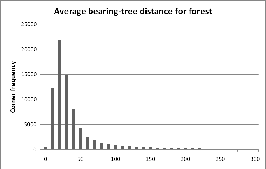
Figure 1. Frequency of 'forest' survey corners in 10-link distance classes by rounding mean distance (e.g., the 10-link class includes corners with mean distance of 5-15 links).
In Figure 1 about 80% of all corners fall in the first 6 classes (up to 55 links). The mean distance for all forest corners is 50 links. Our interpretation is that somewhere around the mean there is a change in the nature of the distribution. Classes under 50 links are common and likely represent the natural range of variation in stocking (perhaps due to age). Classes over 50 links are infrequent and most likely represent a corner where at least one quadrant lacked nearby trees or had damaged trees due to disturbance. Thus, for our 'undisturbed' wooded and riverine classes, it just turns out that the mean distance usually falls in the last or one of the last abundant distance classes, and classes with longer distances were assumed to be disturbed to some extent. To make a simple rule, we arbitrarily set the minimum distance indication disturbance to the mean for vegetation that the surveyors described as swamp, forest, dry ridge, grove, island, bottomland, or dry land.
Setting the upper limit, above which we assume stand-replacement, was also a guess. It is clear that mean distances over about 180 links are typical of open, treeless environments (Table 1.). Even at distances of about 110-180 links it is clear that trees were scarce enough that the surveyors noted that the vegetation wasn't forest. The distribution in Figure 1 is incredibly smooth over the longer mean-distance classes and there is no gap in classes to suggest a natural break for our higher distance threshold. To make a simple rule, we arbitrarily set the maximum distance indicating stand-replacing disturbance as the mean plus one standard deviation for swamp, forest, dry ridge, grove, island, bottomland, or dry land. For most classes, this number is close to the mean distances for open types that we know had very few trees.
The frequency distributions of fire-maintained types are different from the wooded and riverine types. At distances greater than the peak class, the fall in frequency is nearly linear, an example of which is for oak openings (Figure 2.). There is no obvious point of inflection to set the lower, naturally-stocked, undisturbed limit, nor are there breaks in the distribution that can help us set the upper limit for catastrophic disturbance. It is important to remember that we are interpreting the use of terms like 'openings' and 'scatterings' to corners that we believe from modern vegetation to be capable of forest stocking. Almost certainly, these terms were used to describe recent disturbance that caused trees to be sparser than normal 'forest.' To help us interpret the use of these terms to describe forest, we returned to the coarser analysis. Corners with distances under 50 links were almost certainly in places one would describe as undisturbed forest. Corners with distances over 200 links were in places where tree density was low and comparable to open habitats like prairie and meadow. To make a simple rule for corners described as thicket, pine openings, oak openings, scattering timber, and barrens, we arbitrarily set the minimum distance indicating disturbance to 50 links, and we set the maximum distance indicating stand-replacing disturbance at 200 links.
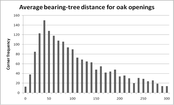
Figure 2. Frequency of 'oak opening' survey corners in 10-link distance classes by rounding mean distance (e.g., the 10-link class includes corners with mean distance of 5-15 links).
In addition to distance, we found it important to consider also missing bearing trees as evidence of disturbance. A common survey note is 'NOTA' meaning 'no other tree around,' which was the surveyor's explanation for not marking all of the required bearing trees (i.e., 4 at section corners and 2 at quarter-section corners). Most often this note appeared at corners described as one of the fire-maintained or open community groups (Table 1.). NOTA was also used at corners described as burned or windthrown. Within the context of interpreting corners modeled as forest or woodland, NOTA almost certainly was relating to some kind of disturbance that left dead trees or trees too small to scribe. Table 2 describes our model for assigning a disturbance class based on both distance and complement of bearing trees. Within their type, survey corners were assigned their final disturbance class -- undisturbed, partially disturbed, catastrophically disturbed -- by a combination of the corner's mean distance to its bearing trees and whether it had its full complement of 2 or 4 bearing trees.
Assumed undisturbed - Wooded and Riverine groups
< mean
between mean and mean + SD
>Mean + SD
Full complement
Undisturbed
Undisturbed
Maintenance
Partial complement
Undisturbed
Maintenance
Burned
Assumed disturbed - Fire-maintained group
< 50 links
links
> 206 links
Full complement
Undisturbed
Maintenance
Burned
Partial complement
Maintenance
Maintenance
Burned
Table 2. Rules for assigning a disturbance class to survey corners not explicitly described as burned or windthrown.
Adjusting the Model -- Window of Recognition
It is obvious that several pragmatic decisions and rules were made in order to assign corners to disturbance categories. Even if these rules are reasonable, one must still set a 'window of recognition' in order to make quantitative estimates of stand-replacing and maintenance rotations. The window of recognition is the span of years for which a surveyor would have bothered to describe a disturbance. Would a surveyor recognize and care to report that a stand had been burned 5, 10, 15, or 20 years after the fact? We believe that mention of fire and windthrow was more an excuse for not marking bearing trees than any conscientious effort to alert potential buyers to fire- or wind-damaged timber. Consider the fact that quaking aspen is the early successional species for nearly all terrestrial forests in Minnesota. The surveyors actually marked and scribed some 390, 2-inch aspen bearing trees and some 3,039 three-inch trees. Clearly, surveyors would bother to scribe 2-3' trees if that was their only choice. Our age/diameter models for 2-3' aspen trees suggest that these trees were between 11 and 18 years old respectively. If commenting about fire and wind was an excuse, then the window of recognition should be somewhere in the 11-18 year range because that is when trees reach a minimum diameter for marking.Alternatively, a window of recognition is empirically set to 'force' the rotation model to match the estimates from studies using more reliable methods. In the Great Lakes States, there are reconstructions of disturbance regimes from fire-scar studies (Frissell 1973), stand-origin mapping (Heinselman 1996), and charcoal analysis of varved sediments (Clark 1988). When we model disturbance regimes from bearing trees in these same regions, a window of 15 years tends to yield results similar to the other methods for stand-replacing disturbance. We used a 15-year window of recognition because it yields rotations comparable to rotations calculated from fire-scars, stand-origin maps, and varved lake sediments.
Many detailed investigations of forest disturbance do not calculate rotations of maintenance disturbance, but recognize its confounding effect on estimating stand-replacing events. Trees with multiple fire-scars attest that some forest types are affected more by maintenance surface fire than catastrophic crown fires. Dendrochronological reconstructions of stand history also attest that maintenance events (fire and non-fire) are common and important, releasing cohorts of advance regeneration and providing some growing space in the canopy (e.g. Bergeron et al. 2002). Minor peaks in varve charcoal are also more common than major ones, possibly recording maintenance fires. Calculating maintenance disturbance is more complicated than stand-replacement because the signal is weaker, reliable studies are fewer, and the cause less obvious. However, some estimate is absolutely required to provide guidance in applying intermediate silvicultural treatments to the right NPCs.
As was the case for estimating stand-replacing rotations, adjusting the window of recognition is the easiest way to adjust the model. Logic would suggest that the window should be shorter for maintenance events because the disturbance is less intense and evidence of it might be gone in 15 years. If the surveyors really used terms like burned or windthrown to explain the lack of bearing trees, it is likely that they did so less often on lands lightly disturbed because there were trees around -- they just had to go a little farther to find bearing trees and might not always find a suitable tree in all quadrants. We found that a 5-year window produced rotations that matched what one might guess from multiple-scarred trees. Also, the ratio of maintenance events to catastrophic ones seemed within the range of what one might expect from the ratio of strong charcoal peaks to minor ones in varve studies. A 5-year recognition window was used to calculate maintenance rotations because it seems to fit fire-scar and varve studies.
Calculating Rotation by Example -- Northern Mesic Mixed Forest (FDn43)
Having settled on windows of recognition and having assigned disturbance classes to the corners associated with an NPC, it is possible to calculate rotation. This is easiest to understand by example.Northern Mesic Mixed Forest (FDn43) is a fire-dependant NPC that is the matrix vegetation for much of northeastern Minnesota. Our model assigned 11,712 PLS survey corners to this community because 1) they fall on landforms (LTAs) where we have modern samples of FDn43 forests, 2) the attending bearing trees were typical of the community (>70% frequency), and 3) they lacked trees atypical of the community (<30% frequency).
Each corner was assigned one of 4 disturbance classes based upon the distance and complement rules set up for each physiognomic vegetation class (Table 2.). The tallies for each class are shown in Table 3.
Vegetation Class
Fire 15-year window
Wind 15-year window
Maintenance 5-year window
Undisturbed
Barrens
11
11
Dry ridge
1
29
Forest
42
111
10168
Grove
1
Bottoms
45
Scattering pine
7
16
Scattering timber
2
24
60
Swamp (misassigned)
5
153
Thicket
21
61
143
Burned
710
Ravine
6
Windthrown
63
No other tree around
16
Island
1
5
Totals
791
63
221
10637
Table 3. Counts of survey corner assignment to disturbance classes by physiognomic vegetation class for the FDn43 community.
The FDn43 landscape of 11,712 survey corners provides the base area for calculating rotation of a NPC. In Table 3, 791 of those corners were interpreted as having been catastrophically burned, representing 6.75% of the area.
(791 burned corners/11,712 total corners)*100=6.75% of the landscapePresumably, surveyors recognized burned lands for 15 years after the event, meaning that the annual percent of the landscape that catastrophically burned is 1/15th of 6.75%.
6.75% of landscape burned/15-year recognition window=0.45% burned annuallyThe rotation is the time required to catastrophically burn the entire area represented by 11,712 corners. Because we have calculated this as a percent, the time it takes to achieve that is:
100%/0.45% burning annually=222 year rotation of catastrophic fireThere is no need to calculate acres or percent of landscape, but it makes the calculation easier to understand given the area concept of rotation in forestry. The easier formulas to use are:
(Total # corners / # corners in disturbance category)*recognition window=rotation
(11,712/791burned)*15 years=222 year rotation of catastrophic fire
(11,712/63 windthrown)*15 years=2,788 year rotation of catastrophic windthrow
(11,712/221 maintenance)*5 years=265 year rotation of maintenance disturbanceIt is also useful to calculate the rotation of all fire (or wind), regardless if it was catastrophic or maintenance. To make this calculation it is easiest to sum the annual percents.
0.45% burned catastrophically each year
0.37% burned in maintenance event
0.45%+0.37%=0.82% annual=122 year rotation for all types of firesIt is the rotation of all fires that tends to reasonably match the published estimates of return intervals. For example, in the BWCAW Heinselman (1996) reports return intervals for the common forest types: Aspen-Birch-Conifer (70-110 years), Red Pine (<100), and White Pine (>100). These cover types, especially the white pine, are predominantly the FDn43 community for which we calculate a 122 year rotation for all fires.
The table below shows the frequency of PLS survey corners assigned to four different disturbance categories. Shown also is the percent of the WFs57 landscape in those conditions and the resulting calculated rotation. Maintenance disturbances were the most frequent disturbance type. There is no evidence of stand re-initiating fire disturbances.
| WFs57 forest | Fire | Wind | Maintenance | Undisturbed |
|---|
Stand dynamics and growth stages
Understanding natural stand dynamics is the essence of prescription writing. Without some understanding of how dynamics affect tree establishment, thinning, recruitment, competitive ability, form, longevity, and succession during 'unsupervised' stand maturation — foresters cannot write worthwhile prescriptions. For the most part, prescriptions are written to re-initiate, transition, or maintain the natural course of events in a forest in order to meet a management objective.
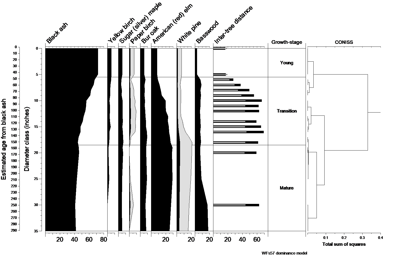
Public land survey records were used to develop a natural model of compositional succession and structural change. The figure below orders PLS section and quarter-sections by diameter class, assigned as the diameter of the largest attending bearing tree at the corner. Presumably this is chronological ranking along the y-axis. The rough age of each diameter class was estimated by FIA diameter/age models for a tree common in all diameter classes.
For every tree, its relative abundance in a diameter class is graphed along the x-axis. This shows the compositional change as forests mature from small diameter classes to larger ones. The inter-tree distances provide some insight concerning initial tree density and how that changes as forests age. Low standard deviation of the inter-tree distances indicate uniform tree spacing; high standard deviations indicate a patchy distribution of trees. A cluster analysis (CONISS) groups contiguous diameter classes into periods of stability (growth-stages) and change (transitions).
- Learn more about natural dynamics and growth stages
Stand Dynamics
PLS data are not inherently temporal. To create a model of stand dynamics we must somehow rank survey corners assigned to a particular NPC Class in a way that is reflective of time. The best that can be done is to assign each corner to a diameter-class equal to the diameter of the largest bearing tree at that corner. This allows us to reasonably rank corners from smaller-diameter/presumably younger forests to larger/presumably older forests the first 100 years or so. We refer to the diameter of the largest tree at a corner as 'stand-diameter.' We believe that this ranking is good enough to make some broad interpretations about dynamics throughout the early years of stand maturation. The modeled age of the largest tree at a corner is a minimum estimate of how long the stand has avoided a catastrophic disturbance. This is NOT true stand age because no corner can be assigned a diameter/age beyond the biological size or longevity of its old-growth species. For forest classes with long rotations of stand-replacing disturbance, the largest tree at any point can easily belong to the 2nd, 3rd, or subsequent cohort. Survey corners were assigned to 'stand-diameter' classes equal to the diameter of the largest witness tree at that corner.
For the set of corners in a diameter class we calculated the relative abundance of each bearing tree taxon. This allows us to see how composition changes as stand-diameter increases over time. For each tree taxon, we plotted its relative abundance by stand diameter to see if its relative abundance tends to decrease, increase, or peak over the range of stand-diameters (below). Also, for the set of corners in a diameter class we calculated the mean distance of trees to the corner and the standard deviation of that mean. This allows us to understand how tree density and variance in density changes as stand diameter increases over time. Because these dynamic models are useful for forest planning the estimated age of a tree that diameter is provided. This is done for a tree species that is abundant and present in all stand-diameter classes. The model is based upon diameter and age measurements of FIA site trees. Stand diameter age was estimated by using a quadratic equation that was fit to FIA site-index trees.
Age=C+A*dbh+B*dbh2 (where C is a constant, A&B are coefficients from the FIA model)
A constrained clustering routine (CONISS, constrained incremental sum of squares) was applied to the stand-diameter classes as characterized by the relative abundance of trees in that class. This method is constrained in that stand-diameter classes must be grouped to its adjoining classes or clusters that include the adjoining classes. The result is a hierarchical grouping of contiguous diameter classes based upon the similarity of their tree composition (below). Tight groups represent a span of stand-diameters where we infer little compositional change. We call these 'growth-stages.' Separating growth-stages are clusters of contiguous diameter classes that are not necessarily very similar, but are the last to be clustered. Such spans of diameter classes represent periods of species turnover called 'transitions.' This analysis provides some insight into the timing and rate of dynamic change.
Graphed for each of the common WFs57 trees is their relative abundance (percent composition; x-axis) as PLS bearing trees by diameter class. In cases where the PLS surveyors did not distinguish species common to the WFs57 community, the more probable species is the graph title and the less probable species is shown in parentheses (e.g. Sugar (silver) maple). Also shown is the mean distance of trees to the survey corner (inter-tree distance, white inset bars) and the standard deviation about that mean (black bars) for each diameter class. All data were smoothed using a 5-sample running average. Curves for taxa not exceeding 5% have a shaded 5X exaggeration to better illustrate trends (e.g. Paper birch). A constrained cluster analysis (CONISS) groups diameter classes with similar species composition; the groups are interpreted as either stable growth-stages (e.g. young, mature) or periods of change (transition). Data for WFs57 comprise 1,109 PLS corners and 3,217 witness trees.
Natural dynamics model for WFs57
Compositional Succession
WFs57 forests were among several wetland communities where a particular hydrologic regime translated into dominance by a single species. If other species occurred it is due to slight topographic variability or spatial variation of the site’s hydrology. In this case, upwelling groundwater strongly favored black ash. However, WFs57 sites were spatially complex with spring heads, spring runs, peaty swales, exposed alluvium, and often ridges or islands of wet mineral soil. The drier portions of these sites reflected the composition of the surrounding mesic hardwood forests and southern terrace forests, and thus compositional succession appeared to follow the tolerance-model typical of the adjacent hardwood forests. The peaty portions of young WFs57 forests were strongly dominated by black ash, and it seems unlikely that much compositional succession occurred. Disturbances that resulted in stand re-initiation left young WFs57 forests that were dominated by black ash. All other species suited to WFs57 sites were also present in the initial cohort, but were minor components. Succession was driven by a long and gradual replacement of mid-tolerant black ash with more tolerant American or red elm and basswood. Most compositional change occurred over the period when stand diameter increased from 5-18 inches. By the time stand diameter reached 18 inches and the forest was about 150 years old, most canopy trees belonged to the second cohort. From that point forward stands were compositionally stable with black ash accounting for about half of the trees, and the remainder was a mixture of hardwoods including: American elm, sugar maple, bur oak, basswood, and some white pine. Sugar or silver maple and bur oak showed little change in abundance throughout stand maturation and it is likely that they occupied mineral inclusions that were not subject to the disturbance agent that affected the ash-dominated portions of these sites.
Structural Succession
Structural succession in WFs57 forests was typical of wet forests in general. In the course of stand maturation they changed considerably with regard to tree density and the evenness at which trees were distributed. Change was rapid due mostly to the presence of all suitable species in the initial cohort, and wider spacing as trees grew to large diameter and expanded their crowns. By the time stand diameter reached 4-5 inches any self-thinning was essentially complete and trees of the young forest were just 18 feet apart, which is typical of northern wet forests and far denser than any young forests in the surrounding, upland landscape. Tree spacing increased dramatically to about 43 feet over the period when stand diameter increased from 5-9 inches. Inter-tree distance changed little from that point on. This decrease in density coincided with the decline of initial cohort black ash, and immediate replacement by American or red elm and basswood. The distance of 43 feet in the late-transition and at maturity was greater than that typical of northern black ash swamps and is comparable to southern hardwoods and southern terrace forests. Thus when young, WFs57 forests were stocked much like a northern wet forest, but when mature, tree spacing more resembled that of southern hardwoods.
WFs57 forests also showed considerable variance in tree spacing as stands aged. Young forests were uniform having ratios of standard deviations to mean inter-tree distances of about 0.9. Over the period when stand diameter increased from 6-9 inches this ratio increased and peaked at about 1.4. This tendency of a patchier distribution of trees coincides with the decline of black ash and was likely due to the creation of large canopy gaps as initial cohort ash died. After stand diameter reached 10 inches WFs57 stands remained patchy, and the ratio of standard deviations to their inter-tree means ranged between 1.3 and 1.4. This suggests that the formation of both large and small canopy gaps provided recruitment opportunities in mature forests for the full suite of WFs57 trees.
Silvicultural strategies
Silvicultural strategies are sequences of treatment outcomes designed to emulate natural stand dynamics and promote natural regeneration. They are not silvicultural systems in the traditional sense because they do not cover a full rotation or have attached the implied goal of maintaining a particular species or cover-type indefinitely. Most involve 1-2 stand entries over a short period of time that will move a stand towards a forest plan objective -- with enough inertia that little silvicultural intervention will be needed to meet long-term goals. We describe management outcomes rather than silvicultural treatments because there are usually several treatments that might achieve the desired outcome. All strategies are based upon our understanding of NPC-specific natural stand dynamics and disturbance regimes. The sequence of outcomes follows the natural pattern; the timing is foreshortened because we intend to harvest sound trees rather than allowing natural senescence.
The most common, natural pattern of tree mortality and replacement was the partial loss of trees on a rotation of about 140 years. Stand-replacing windthrow was infrequent with an estimated rotation of 630 years. There is no evidence of stand-replacing fire in the PLS field notes.
Unlike wetlands that accumulate runoff, WFs57 forests are wet due to groundwater discharge and a stable water table near the soil surface. Such areas tend to be hydrologically stable because it takes some time for water to infiltrate, reach an aquifer and move downslope to the wet black ash forest. Thus the hydrology of these sites doesn’t change in response to single storms and probably doesn’t change much regarding seasonal differences in precipitation. Landscape variables such as annual precipitation, the size of the catchment, infiltration rates of the soils within the catchment, hydraulic conductivity of the aquifer, confinement of the aquifer, slope and head, etc. determine for the most part just how responsive a particular WFs57 forest will be to changes in water input. The contributing landscape to any particular forest is unknown and likely unique. While, long-term fluctuations in hydrology probably killed black ash trees and resulted in stand re-initiation, it cannot be silviculturally emulated.
Windthrow was the natural agent of tree mortality and that only occasionally resulted in stand re-initiation. Partial windthrow is evident in nearly all modern examples of WFs57 forests, particularly where the soils are peaty, constantly saturated, and structurally weak. The spring heads, spring runs, and zones of active seepage rarely, if ever freeze to the point where logging or other management is a viable option. Furthermore, these sites harbor some of the state’s rarer plants. WFs57 forests themselves are rare inclusions within a matrix of more manageable hardwood and terrace forests. Management should focus on the conservation of WFs57 forests and protection of their hydrologic situation.